R 데이터 시각화 (그래프 3)

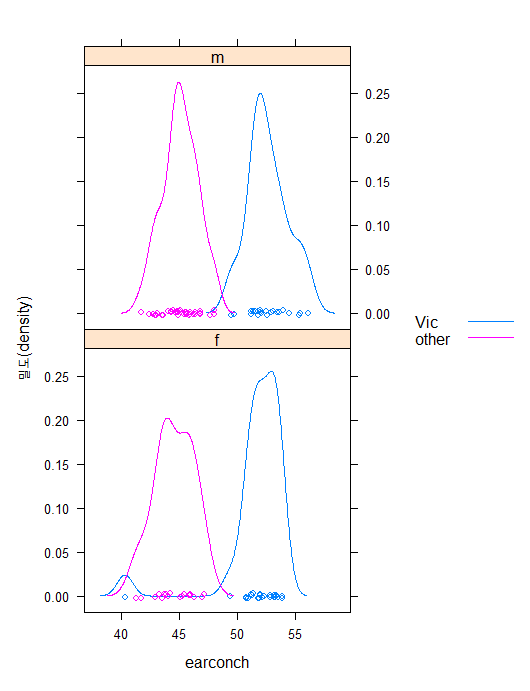
> ## Density plot for earconch: data frame possum (DAAG package)
> library(DAAG)
> library(lattice)
> densityplot(~earconch | sex, groups=Pop, data=possum,
+             auto.key=list(space="right"))
> 
> ## Apply function range to columns of data frame jobs (DAAG)
> sapply(jobs, range)
       BC Alberta Prairies Ontario Quebec Atlantic     Date
[1,] 1737    1366      973    5212   3167      941 95.00000
[2,] 1840    1436      999    5360   3257      968 96.91667
> 
> 
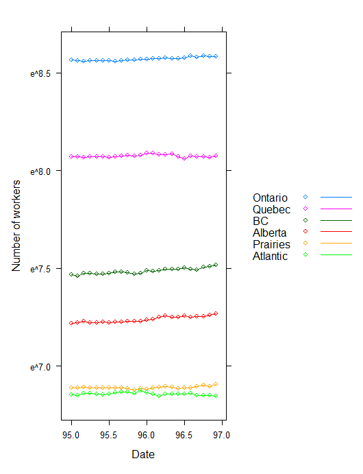
> ## Simplified plot; all series in a single panel; use log scale
> (simplejobsA.xyplot <-
+         xyplot(Ontario+Quebec+BC+Alberta+Prairies+Atlantic ~ Date,
+                outer=FALSE, data=jobs, type="b",
+                ylab="Number of workers", scales=list(y=list(log="e")),
+                auto.key=list(space="right", lines=TRUE)))
> 
> 
> ## Simplified code for Figure 2.9B
> xyplot(Ontario+Quebec+BC+Alberta+Prairies+Atlantic ~ Date,
+        data=jobs, type="b", layout=c(3,2), ylab="Number of jobs",
+        scales=list(y=list(relation="sliced", log=TRUE)),
+        outer=TRUE)
> 
> 
> (target.xyplot <-
+         xyplot(csoa ~ it | sex*agegp, data=tinting, groups=target,
+                auto.key=list(columns=2)))
> 
> (tint.xyplot <-
+         xyplot(csoa ~ it|sex*agegp, groups=tint, data=tinting,
+                type=c("p","smooth"), span=1.25, auto.key=list(columns=3)))
> # "p": points; "smooth": a smooth curve
> # With span=1.25, the smooth curve is close to a straight line
> 
> 
> 
> ## Panel B, with refinements
> themeB <- simpleTheme(col=c("skyblue1", "skyblue4")[c(2,1,2)], lwd=c(1,1,2),
+                       pch=c(1,16,16)) # open, filled, filled
> update(tint.xyplot, par.settings=themeB, legend=NULL,
+        auto.key=list(columns=3, points=TRUE, lines=TRUE))
> # Set legend=NULL to allow new use of auto.key
> 
> ## Table of counts example: data frame nswpsid1 (DAAG)
> tab <- with(nswpsid1, table(trt, nodeg, useNA="ifany"))
> dimnames(tab) <- list(trt=c("none", "training"),
+                       educ = c("completed", "dropout"))
> tab
          educ
trt        completed dropout
  none          1730     760
  training        80     217
> 
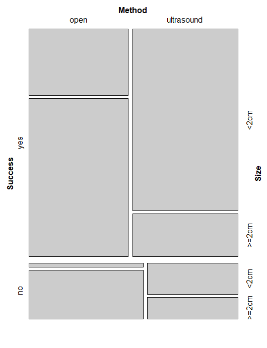
> stones <- array(c(81,6,234,36,192,71,55,25), dim=c(2,2,2),
+                 dimnames=list(Success=c("yes","no"),
+                               Method=c("open","ultrasound"),
+                               Size=c("<2cm", ">=2cm")))
> # NB: The margins are 1:Success, 2:Method, 3:Size
> library(vcd)
필요한 패키지를 로딩중입니다: grid
> mosaic(stones, sort=3:1) # c.f. mosaicplot() in base graphics
> # Re-ordering the margins gives a more interpretable plot.
> 
> ## Function to calculate percentage success rates
> roundpc <- function(x)round(100*x[1]/sum(x), 1)
> ## Add "%Yes" to margin 1 (Success) of the table
> stonesplus <- addmargins(stones, margin=1, FUN=c("%Yes"=roundpc))
> ## Print table, use layout similar to that shown alongside plot
> ftable(stonesplus, col.vars=1)
                 Success   yes    no  %Yes
Method     Size                           
open       <2cm           81.0   6.0  93.1
           >=2cm         192.0  71.0  73.0
ultrasound <2cm          234.0  36.0  86.7
           >=2cm          55.0  25.0  68.8
> ## Get sum for each margin 1,2 combination; i.e., sum over margin 3
> stones12 <- margin.table(stones, margin=c(1,2))
> stones12plus <- addmargins(stones12, margin=1, FUN=c("%Yes"=roundpc))
> ftable(stones12plus, col.vars=1) # Table based on sums over Size
           Success   yes    no  %Yes
Method                              
open               273.0  77.0  78.0
ultrasound         289.0  61.0  82.6